ポーズ推定を使ってピクトさんを量産する

その昔、画像から人のポーズ推定ができたら、ピクトさんの画像が大量に作れるなーと考えたことがありました。当時は諦めましたが、ここ最近のDeep Learning技術の発展で実現の可能性が出てきました。少し前に Realtime Multi-Person Pose EstiamtionのChainer実装が公開されていたので、ありがたく使わせてもらって、「写真からピクトさんを生成する」をやってみます。なお、この記事の環境構築から後の部分はJupyter Notebookでそのまま動くようにしてあるので、興味を持たれた方はそのままコピペして実行して見てください。

Contents

やること
環境構築
マニュアルで推論を行う
図形を描画する関数を準備しておく
ピクトさんの描画
他の画像で試してみる
まとめ

やること

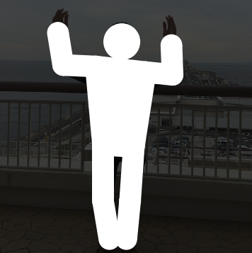
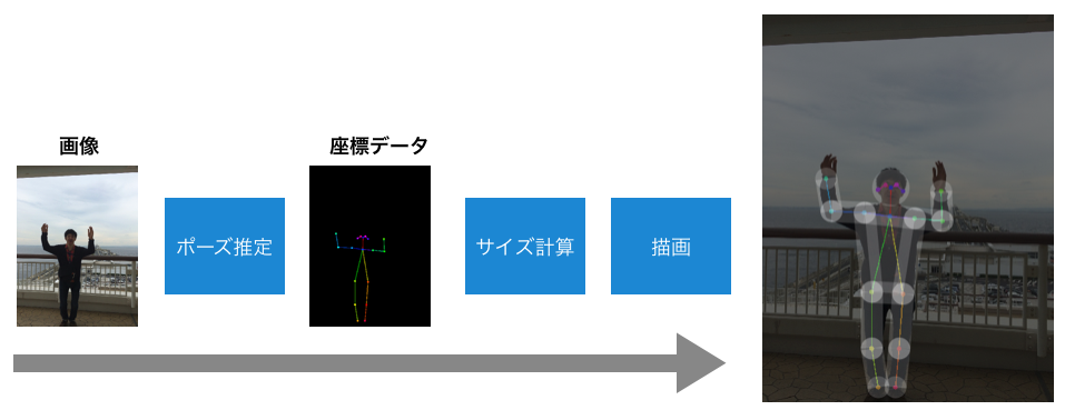
「写真からピクトさんを生成する」がこの記事のゴールになります。まず、今回やることの全体像を示しておきます。なお、図の一番右の画像はわかりやすさのために半透明にしていますが、白一色で塗りつぶします。

内容としては、

最初に、学習済みのモデルを使ってポーズ推定を行います。
得られた座標データから、頭のサイズや腕・足の太さを計算する
描画する

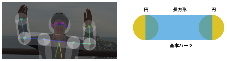
といった感じです。ポーズ推定から得られるのは鼻や肘といったキーポイントの座標データのみなので、それをピクトさんらしく見せるのには一工夫が必要です。今回は、以下のように、円と長方形を組み合わせて描画を行います。

環境構築

それでは最初に、ピクトさん生成のための環境を構築します。基本は、ポーズ推定のChainer実装のREADMEにある依存ライブラリのインストールですが、Jupyter Notebookで作業するのでそれも先に入れておきます。

前提（というか手元の環境）：

Python 3.5.1 (READMEを読むと3系なら大丈夫なようです。）
pipが使える

まずは pip コマンドで必要なライブラリのインストールです。ちなみに、記事執筆時点では、Chainerのバージョンは3.2.0でした。

pip install chainer matplotlib jupyter opencv-python scipy

次に、Chainer版のRealtime Multi-Person Pose Estiamtionのリポジトリをクローンします。

git clone https://github.com/DeNA/Chainer_Realtime_Multi-Person_Pose_Estimation.git

訓練済みのパラメータファイルをダウンロードし、caffemodelからnpzに変換します。

cd Chainer_Realtime_Multi-Person_Pose_Estimation/models
wget http://posefs1.perception.cs.cmu.edu/OpenPose/models/pose/coco/pose_iter_440000.caffemodel
python convert_model.py posenet pose_iter_440000.caffemodel coco_posenet.npz
cd ..

無事に環境構築ができたかどうか、サンプルの推論スクリプトを実行してみます。

MPLBACKEND="agg" python pose_detector.py posenet models/coco_posenet.npz --img data/person.png

result.png というファイルが生成され、正しく関節の位置が推定できていればOKです。

マニュアルで推論を行う

先ほどは付属のスクリプトを実行して関節位置の推定を行いましたが、ここからはJupyter Notebookでコードを書きながらピクトさんの量産を進めていきたいと思います。

ここからは以下のディレクトリを作成し、その中にnotebookを作成して開発を進めていきたいと思います。

Chainer_Realtime_Multi-Person_Pose_Estimation/notebooks

%matplotlib inline

import os
import sys

import cv2
import matplotlib.pyplot as plt
import matplotlib.patches as mpatches
import numpy as np

最初に、chainer版のOpenPoseのモデルをインポートします。

# モジュール検索パスの設定
REPO_ROOT = '..'
sys.path.append(REPO_ROOT)

# PoseDetectorクラスのインポート
from pose_detector import PoseDetector

# モデルのロード
arch_name = 'posenet'
image_path = os.path.join(REPO_ROOT, 'data', 'person.png')
weight_path = os.path.join(REPO_ROOT, 'models', 'coco_posenet.npz')

model = PoseDetector(arch_name, weight_path)

Loading PoseNet...

早速、手元の画像を入力して関節位置の推定をやってみます。まずは入力画像の確認です。

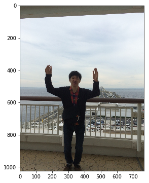
# サンプル画像
img = cv2.imread('../sample_images/sample02.jpg')

plt.figure(figsize=(6, 6))
plt.imshow(img[:, :, ::-1] )  # BGR -> RGB
plt.show()

こんな画像を入力してみます。推論を行うAPIはシンプルになっていて、以下のように実行します。

pose_arr = model(img)

Inference scale: 1.0...

可視化コードも用意してくれているので、認識結果を画像に重ねて表示してみます。

from pose_detector import draw_person_pose

result_img = draw_person_pose(img, pose_arr)

plt.figure(figsize=(6, 6))
plt.imshow(result_img[:, :, ::-1])
plt.show()

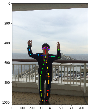
正しく関節の位置を認識できているようです。続いて、認識結果の中身も確認しておきます。

print("type: {}".format(type(pose_arr)))
print("shape: {}".format(pose_arr.shape))
print(pose_arr)

type: <class 'numpy.ndarray'>
shape: (1, 18, 3)
[[[340 457   2]
  [338 533   2]
  [271 523   2]
  [184 519   2]
  [170 433   2]
  [403 538   2]
  [475 545   2]
  [472 466   2]
  [290 732   2]
  [290 881   2]
  [307 983   2]
  [372 737   2]
  [362 881   2]
  [352 983   2]
  [326 450   2]
  [355 450   2]
  [307 462   2]
  [372 466   2]]]

結果は(N, 18, 3)の形状の numpy.ndarray 型となっており、以下のような情報が格納されている

Nは検出した人数（今回は一人）
18は関節の数で固定。順に鼻、首、…のように定義されている
3はX座標、Y座標、フラグとなっており、関節が見つからない場合はフラグに0の値が入る模様

関節の定義はこちらにあります。

ひとまず、無事に手元の画像を使ってマニュアルで人の姿勢推定を動かすことができました。

図形を描画する関数を準備しておく

冒頭に述べた通り、円と長方形を組み合わせて描画をしていきます。 matplotlib.patches を使って描画していくことにしたのですが、これが簡単に実現できる機能がパッとは見当たらず。仕方がないので自力実装です。まずは以下の図の青色部分の四角形を描画するコードを準備します。

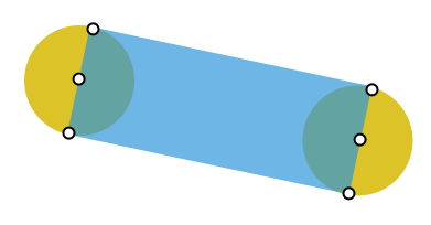
def _draw_line(ax, start, end, radius, **style):
    vec = end - start
    d = np.sqrt(np.sum(vec ** 2))
    cos = vec[0] / d
    sin = vec[1] / d

    corners = np.array([
        [start[0] + radius * sin, start[1] - radius * cos],
        [start[0] - radius * sin, start[1] + radius * cos],
        [end[0] - radius * sin, end[1] + radius * cos],
        [end[0] + radius * sin, end[1] - radius * cos],
    ])

    style = style.copy()
    style['fill'] = True
    ax.add_patch(mpatches.Polygon(corners, **style))
    return ax

次に、円と長方形を組み合わせてピクトさんのパーツ（頭、腕など）を描画する関数を定義します。

def draw_polygon(ax, xy_mat, radius, close_path_and_fill=False, **style):
    xy_prev = None
    for xy in xy_mat:
        ax.add_patch(mpatches.Circle(xy, radius, **style))

        if xy_prev is not None:
            ax = _draw_line(ax, xy_prev, xy, radius, **style)
        xy_prev = xy

    if close_path_and_fill:
        # close path
        ax = _draw_line(ax, xy_prev, xy_mat[0], radius, **style)

        # fill inner area of polygon
        style = style.copy()
        style['fill'] = True
        ax.add_patch(mpatches.Polygon(xy_mat, **style))

    return ax

これで準備完了です。簡単に使い方を紹介しておきます。

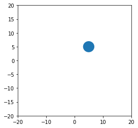
# 確認用のユーティリティ
def display_polygon(xy_mat, radius=2, close_path_and_fill=False):
    fig, ax = plt.subplots(figsize=(4, 4))
    ax.set_xlim(-20, 20)
    ax.set_ylim(-20, 20)
    ax = draw_polygon(ax, xy_mat, radius,
                      close_path_and_fill=close_path_and_fill)
    plt.show()

座標が一つの場合は点（というか円）になります。頭の描画に使います。

# 座標がひとつの場合 -> 頭
xy_mat = np.array([[5, 5]])
display_polygon(xy_mat)

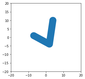
複数の点を渡すと折れ線になります。腕、足用。

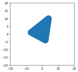
# 座標が複数の場合 -> 腕、足
xy_mat = np.array([[-7, 1], [2, -4], [4, 10]])
display_polygon(xy_mat)

close_path_and_fill にTrueを渡すとパスを閉じて中を塗りつぶします。体部分の描画に使います。

# 塗りつぶし -> 体
xy_mat = np.array([[-7, 1], [2, -4], [4, 10]])
display_polygon(xy_mat, close_path_and_fill=True)

ピクトさんの描画

さて、いよいよ本題です。推定したポーズ情報と準備した描画関数を使ってピクトさんを描画していきます。ここで、２つほど考えておくことがあります。

頭のサイズや線の太さをどう決めるか
関節が見つからない場合はどうするか

まずは頭のサイズの決め方ですが、鼻から首までの距離と、右肩から左肩までの距離を使って推定することにしました。横を向いていると両肩間の距離が小さくなるので、大きい方の値を使っています。 0.38 とか 1.7 はそれっぽく見えるように調整しました。どちらも利用不可能な場合はサイズを None で返し、描画をしないことにします。

def check_availability(pose_data, keypoint_indices):
    result = np.all(pose_data[keypoint_indices, 2] != 0)
    return result

def calculate_reference_size(pose_data):
    distances = []

    # nose - neck
    if check_availability(pose_data, [0, 1]):
        p0 = pose_data[0, :2]
        p1 = pose_data[1, :2]
        d = np.sqrt(np.sum((p1 - p0) ** 2))
        distances.append(d)

    # right shoulder - left shoulder
    if check_availability(pose_data, [2, 5]):
        p2 = pose_data[2, :2]
        p5 = pose_data[5, :2]
        d = np.sqrt(np.sum((p5 - p2) ** 2)) / 2.
        distances.append(d)

    if not distances:
        return None

    ref_size = np.max(distances) * 0.38
    return ref_size

いよいよピクトさんの描画関数です。先ほどの ref_size が None で返ってきた場合はその人物の描画をスキップします。各パーツは、必要な関節の座標が利用可能な場合のみ描画するようにしています。

def get_xy_mat(pose_data, indices):
    xy_mat = pose_data[indices, :2]
    return xy_mat

def draw_pictosan(ax, pose_data, **style):
    ref_size = calculate_reference_size(pose_data)

    if ref_size is None:
        return ax  # skip drawing

    # head
    if check_availability(pose_data, [0]):
        radius = ref_size * 1.7
        draw_polygon(ax,
                     get_xy_mat(pose_data, [0]),
                     radius, **style)

    # body
    if check_availability(pose_data, [2, 5, 11, 8]):
        draw_polygon(ax,
                     get_xy_mat(pose_data, [2, 5, 11, 8]),
                     ref_size, close_path_and_fill=True, **style)

    # arm and leg
    def _draw_arm_or_leg(i1, i2, i3):
        if check_availability(pose_data, [i1, i2]):
            draw_polygon(ax,
                         get_xy_mat(pose_data, [i1, i2]),
                         ref_size, **style)
            if check_availability(pose_data, [i3]):
                draw_polygon(ax,
                             get_xy_mat(pose_data, [i2, i3]),
                             ref_size, **style)
    _draw_arm_or_leg(2, 3, 4)
    _draw_arm_or_leg(5, 6, 7)
    _draw_arm_or_leg(8, 9, 10)
    _draw_arm_or_leg(11, 12, 13)

    return ax

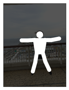
それでは先ほど認識したポーズデータを使ってピクトさんを描画してみます。

style={'facecolor': 'white'}

fig, ax = plt.subplots(figsize=(10, 10))
ax.imshow(img[:, :, ::-1] // 3)

for pose_data in pose_arr:
    draw_pictosan(ax, pose_data, **style)
plt.show()

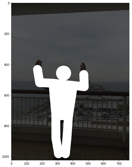
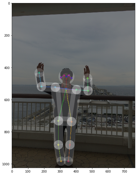
良い感じ。まさにやりたかったピクトさんの描画ができました。ついでにピクトさんを半透明にし、認識結果もセットで表示してみます。

style={'facecolor': 'white', 'alpha': 0.2}

fig, ax = plt.subplots(figsize=(10, 10))
result_img = draw_person_pose(img, pose_arr)
ax.imshow(result_img[:, :, ::-1] //2)

for pose_data in pose_arr:
    draw_pictosan(ax, pose_data, **style)
plt.show()

他の画像で試してみる

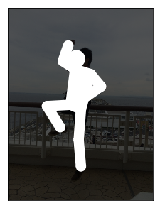
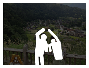
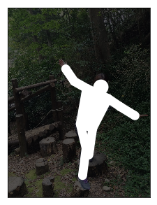
せっかく写真からピクトさんの生成ができるようになったので、何枚か写真を入れて描画して見ます。今回、 sample_images というディレクトリを作成し、その中に何枚か画像を入れています。ぜひお手元の画像で試して見てください。

まずは画像のパス一覧を取得します。

image_dir = os.path.join('..', 'sample_images')
image_names = sorted(os.listdir(image_dir))
image_paths = [os.path.join(image_dir, fn) for fn in image_names]
image_paths

['../sample_images/sample01.jpg',
 '../sample_images/sample02.jpg',
 '../sample_images/sample03.jpg',
 '../sample_images/sample04.jpg',
 '../sample_images/sample05.jpg',
 '../sample_images/sample06.jpg',
 '../sample_images/sample07.jpg',
 '../sample_images/sample08.jpg',
 '../sample_images/sample09.jpg',
 '../sample_images/sample10.jpg',
 '../sample_images/sample11.jpg',
 '../sample_images/sample12.jpg',
 '../sample_images/sample13.jpg']

あとは１枚ずつ画像を読み込んで、ポーズ推定して可視化というのをやっていきます。

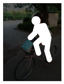
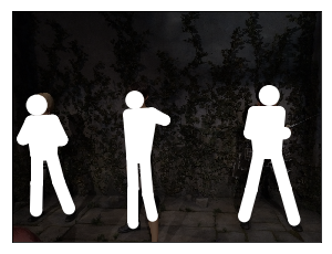
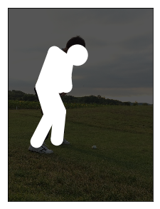
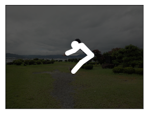
for i, img_path in enumerate(image_paths):
    print('[{}/{}] {}'.format(i + 1, len(image_paths), img_path))
    img = cv2.imread(img_path)
    pose_arr = model(img)

    fig, ax = plt.subplots(figsize=(5, 5))
    ax.imshow(img[:, :, ::-1] // 3)
    ax.set_xticks([])
    ax.set_yticks([])

    for data in pose_arr:
        draw_pictosan(ax, data, facecolor='white')
    plt.show()

[1/13] ../sample_images/sample01.jpg
Inference scale: 1.0...

[2/13] ../sample_images/sample02.jpg
Inference scale: 1.0...

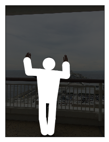
[3/13] ../sample_images/sample03.jpg
Inference scale: 1.0...

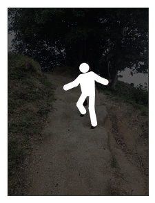
[4/13] ../sample_images/sample04.jpg
Inference scale: 1.0...

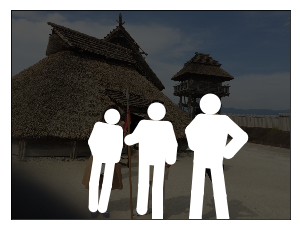
[5/13] ../sample_images/sample05.jpg
Inference scale: 1.0...

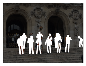
[6/13] ../sample_images/sample06.jpg
Inference scale: 1.0...

[7/13] ../sample_images/sample07.jpg
Inference scale: 1.0...

[8/13] ../sample_images/sample08.jpg
Inference scale: 1.0...

[9/13] ../sample_images/sample09.jpg
Inference scale: 1.0...

[10/13] ../sample_images/sample10.jpg
Inference scale: 1.0...

[11/13] ../sample_images/sample11.jpg
Inference scale: 1.0...

[12/13] ../sample_images/sample12.jpg
Inference scale: 1.0...

[13/13] ../sample_images/sample13.jpg
Inference scale: 1.0...

ちなみに以下のようなコードを書くと、左右に表示できて良い感じです。ご参考まで。

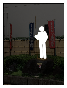
image_paths = image_paths[0:1]

for img_path in image_paths:
    img = cv2.imread(img_path)
    pose_arr = model(img)

    fig, axs = plt.subplots(nrows=1, ncols=2, figsize=(12, 6))

    # original image
    ax = axs[0]
    ax.set_xticks([])
    ax.set_yticks([])
    ax.imshow(img[:, :, ::-1])

    # picto-san
    ax = axs[1]
    ax.imshow(img[:, :, ::-1] * 0)
    ax.set_xticks([])
    ax.set_yticks([])

    for data in pose_arr:
        draw_pictosan(ax, data, facecolor='white')
    plt.show()

Inference scale: 1.0...

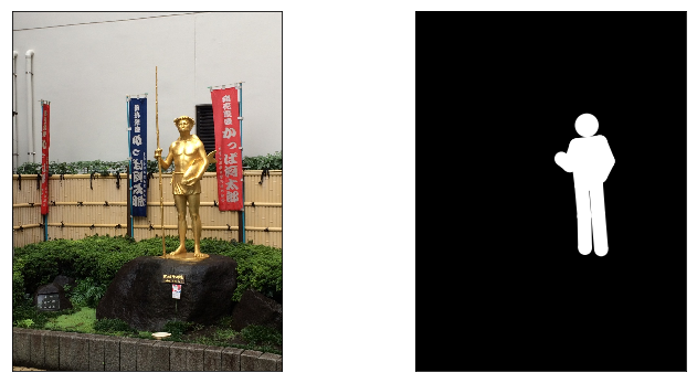
かっぱ橋道具街のかっぱ河太郎さんでした。食器を買いたい方はぜひ、かっぱ橋道具街へ。悪ふざけで入力して見たら完璧にポーズ推定できてちょっとビビりました。

まとめ

ということで、ポーズ推定の結果を使ってピクトさんがつくれるか実験をしてみました。前に思いついたネタがやっと日の目を浴びました。今回は頭の中心座標に「鼻」を使ったので、横を向いている画像だと頭の位置が若干ずれるな、とか、鼻が検知できていないと頭がなくなってホラーだな、、、とか、いろいろ改良の余地はありますが、ひとまずやりたいことが試せたので良しとします。

最後になりますが、Chainer版のRealtime Multi-person Pose Estimationを利用させていただきました。APIが綺麗で使いやすかったです。ありがとうございました。

https://github.com/DeNA/Chainer_Realtime_Multi-Person_Pose_Estimation

ではまた。